Fenwick Trees Are Nothing But…

Introduction #

Most explanations of Fenwick trees — or Binary Indexed Trees — that I’ve seen (some are listed in the references below) describe the data structure in a way that makes it hard to come up with it from scratch.

A good intuitive understanding of a data structure makes it easier to remember and gives you the ability to derive new ones with desired properties. In this post, we’ll consider a very useful visual perspective on Fenwick trees and illustrate its merits by creating a dynamic range minimum queries adaptation.

Segment trees #

In particular, we’ll show how Fenwick trees are in some sense just a cut down version of segment trees.

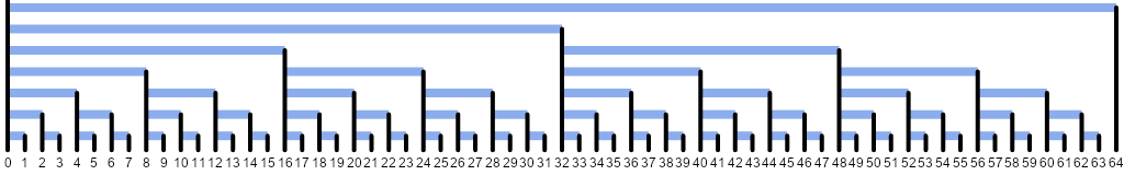
A segment tree divides the array in consideration into two halves, each of which is further divided in half, and so on, until segments of length $1$ are formed. These become the leaves of a binary tree, whose root is a segment covering the entire span of the array and the children of any non-leaf segment are its halves.¹

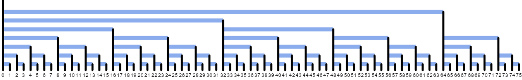
For the number of array elements $n$ that is an integer power of two, the case we’ll focus on for now, this results in an even division each time, producing a structure illustrated below. We mark left children as blue and right children as pink for the reasons that will soon become apparent.² Note how the black divider at a position $x$ rises $h$ levels above the leaves' level where $x = (2k + 1) 2^h$, i.e. $h$ is the largest power of $2$ dividing $x$.

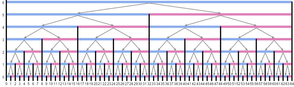
It is immediately obvious that the height of the tree is logarithmic in the number $n = 2^t$ of array elements, since each child half is twice shorter than the parent segment.³ This is reflected in the fact that the tallest divider (except the one at zero that has infinite height) has height $t$.

In order to perform range queries and updates on such a tree, the segment representing the range is split into parts corresponding to the tree nodes. This is typically done in a recursive fashion: starting from the root, the segment in question is either entirely contained in the left or the right child or divided in two at the midpoint separating the children. A crucial observation is that only at most one such division can end up in both subsegments not coinciding with the child segments.

This is illustrated in the following animation, where the left (pink) and right (blue) parts of an initial segment represent the results of such division. As it can be seen, these parts are “stuck” with one end to an endpoint of one of the children on all subsequent levels. Therefore in total there are at most two segment parts of interest at each level, leading to $O(\log n)$ traversal. On the way back, one can recompute segment parameters from those of their children.

Enter Fenwick trees #

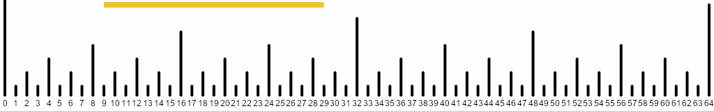
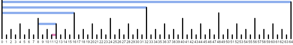
Let’s now focus on those examples where the initial segment already touches the leftmost spike at $0$. Here are specifically such examples: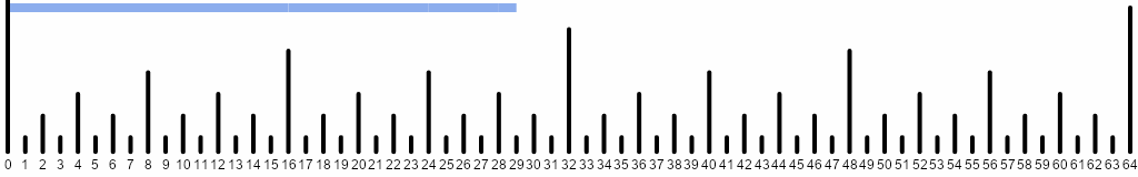

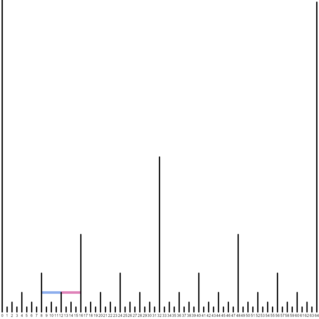
Note that to represent segments of this kind, we only need the blue parts. Each blue segment runs from the tip of a divider spike to the left until it hits a higher spike. Let’s redraw our animation making the length of the divider spikes correspond to the largest power of two dividing their position:

The closest higher spike to the left of a spike at $x = (2k + 1)2^h$ with height $2^h$ is at $k \cdot 2^{h + 1} = 2 k \cdot 2^h = x - 2^h = x - height(x)$, where $height(x)$ is the largest divisor of $x$ that is a power of $2$. Alternatively, it is the value $LSB(x)$ of the least significant bit of $x$; in the ubiquitous two’s complement system for representing negative numbers, $LSB(x) = x \mathop{\&} -x$, where $\&$ is bitwise AND.

Now observe that in order to compute sums on the intervals of the original array, we only need to be able to compute sums on such prefix segments (touching zero), because $sum([l, r)) = sum([0, r)) - sum([0, l))$. This means that of the full segment tree we only need the following segments:

And thus, by associating with each spike a blue segment starting from its tip and going to the left, we can store partial sums on those blue segments. To compute a prefix sum for a given $[0, r)$ segment, we explicitly iterate through the constituent blue segments by repeatedly subtracting $LSB(x)$ from the current right endpoint. This is exactly what a Fenwick tree is about.

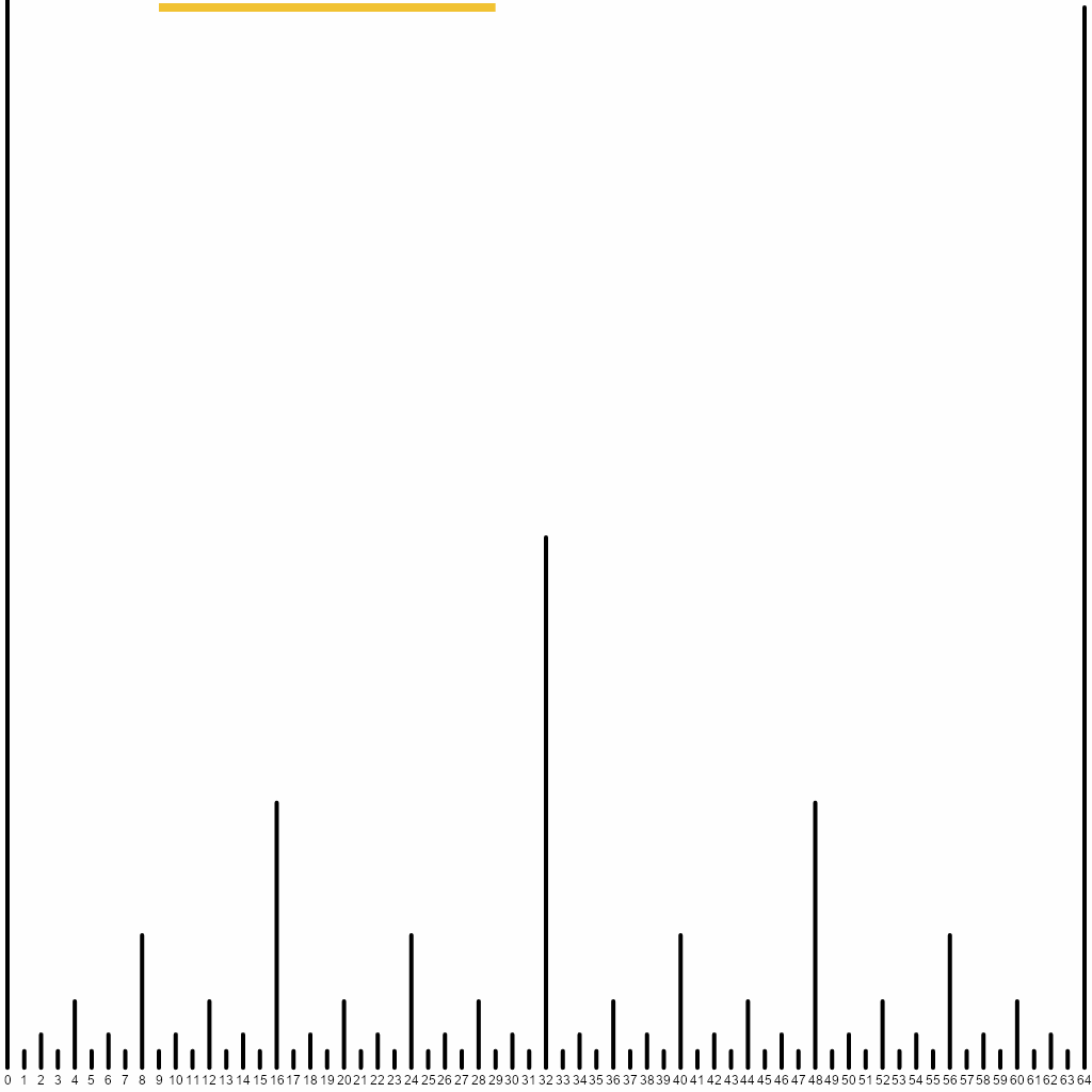
This way, a Fenwick tree can be seen as a certain “half” of a segment tree. Note that for $n$ different from a power of two, a top-down segment tree would arrive at splitting unevenly, whereas a Fenwick tree always splits in the way shown, as if $n$ is rounded up to a power of two. The spikes after $n$ are thrown away afterwards:

We will assume that the array indexing is zero-based; the prefix sum stored in $r$ corresponds to the segment $[r - LSB(r), r)$ of elements $r - LSB(r)$ through $r - 1$ of the original array.

For point updates, one needs to enumerate the spikes whose left partial sums are containing the given array item at index $i$. It’s easy to see that the first such partial sum is stored at $i + 1$. The rest can be found by iterating through subsequently increasing spikes to the right — going from $x = (2k + 1)2^h$ to $x = (2k + 2)2^h = (k + 1)2^{h + 1} = x + 2^h = x + LSB(x)$. Here’s an example of how it looks like when updating the $11$th element, which would be stored in the pink segment $[11, 12)$ if the tree were complete:

For comparison with the later extension of the Fenwick tree, here’s the code. Note the $O(n)$ initialization from a given list of values — it is left as an exercise for the reader to figure it out using the newly acquired visual intuition.

def lsb(x: int) -> int:
    # Note: returns 0 for `x == 0` although it should be infinity.
    #       Therefore `x == 0` should be special-cased in the code.
    return x & -x

class RangeSum:
    def __init__(self, initial_values: Iterable[Number]) -> None:
        values = list(initial_values)
        self.n = len(values)
        self.fenwick = [0] + values  # [0, 0) is an empty segment.
        for pos in range(1, self.n + 1):
            next_ = pos + lsb(pos)
            if next_ <= self.n:
                self.fenwick[next_] += self.fenwick[pos]

    def modify(self, pos: int, add: Number) -> None:
        # We start with updating the segment
        # whose exclusive right end is `pos + 1`.
        pos += 1
        while pos <= self.n:
            self.fenwick[pos] += add
            pos += lsb(pos)

    def query(self, left: int, right: int) -> Number:
        return self._query(right) - self._query(left)

    def _query(self, right: int) -> Number:
        result = 0
        while right > 0:
            result += self.fenwick[right]
            right -= lsb(right)
        return result

This data structure can be used in the CSES problem “Dynamic Range Sum Queries”. (Note that modifications there are absolute rather than relative and the indexing starts from 1, so additional care must be taken on top. Additionally, solutions in Python might need a speedup provided by PyPy in order to fit the time constraints.)

Extending for range minima #

If we want to compute $min([l, r))$, we are out of luck with the approach of the original Fenwick trees. That’s because one cannot reduce computing minima on arbitrary $[l, r)$ segments to those of the $[0, r)$ kind.

But we know that segment trees can be trivially applied to this task. Therefore let’s go back to the original animation and see what we’re missing: it’s precisely all the pink segments! We can also associate them with the spikes on whose tips they rest.

Let’s store minima on blue parts in one array (left) and on pink parts in another (right)⁴. Observe that the underlying (original) array items are stored between the two arrays of our Fenwick structure in the combination of all the length-$1$ blue and pink parts. With a particular divider spike at $x$ we associate two ranges: $[x - LSB(x), x)$ and $[x, x + LSB(x))$. Here they are depicted for $x = 12$:

Back to our segment splitting: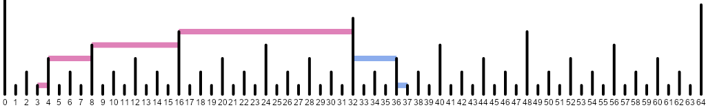

When computing the minimum on the given segment $[l, r)$ (like $[3, 37)$ in the image above), we iterate through the pink segments by repeatedly adding $LSB(current\_l)$ to $current\_l$ (starting from $l$) until it meets or exceeds $r$, and then we iterate through the blue segments by repeatedly subtracting $LSB(current\_r)$ from $current\_r$ (starting from $r$). Note that both processes meet at the first split point of the “falling” segment.

Exercise for the reader: Suppose $l$ is has a binary representation of $\overline{X0Y}_2$ and $r$ is represented as $\overline{X1Z}_2$, where $X$ is their longest common binary prefix and $Y$ and $Z$ are some suffixes of the same length. Show that the first split occurs at $\overline{X10\ldots 0}_2$ and the above iterations from the left and from the right converge at that point.

After a point update, we “climb up” the underlying segment tree, understanding whether the current segment $[l, r)$ is the left or the right child (in the segment tree sense) of its parent by comparing $height(l)$ and $height(r)$. Then the minimum over a parent segment is trivially the minimum between its child segment minima.

Show me the code #

Sure! Here it is:

INF = float('inf')

class RangeMinimum:
    def __init__(self, initial_values: Iterable[Number]) -> None:
        values = list(initial_values)
        self.n = len(values)
        self.left = [INF] + values   # "blue" - left of a spike tip.
        self.right = values + [INF]  # "pink" - right of a spike tip.
        for pos in range(1, self.n + 1):
            next_ = pos + lsb(pos)
            if next_ <= self.n:
                self.left[next_] = min(self.left[next_],
                                       self.left[pos])
        for pos in range(self.n, 0, -1):
            prev = pos - lsb(pos)
            if prev >= 0:
                self.right[prev] = min(self.right[prev],
                                       self.right[pos])

    def modify(self, pos: int, new_value: Number) -> None:
        # Point modification at `pos`
        # is a modification of `[pos, pos + 1)`.
        left = pos
        right = pos + 1
        # Holds the minimum on [left, right).
        min_value = new_value
        # "Climb" up the segment tree.
        while left > 0 or right <= self.n:
            if right <= self.n and (left == 0
                                    or lsb(left) > lsb(right)):
                self.left[right] = min_value
                # We are about to extend the segment to the right,
                # and its new center will be at the current `right`.
                # Include the minimum over its right (pink) part.
                min_value = min(min_value, self.right[right])
                right += lsb(right)
            else:
                # We are about to extend the segment to the left,
                # and its new center will be at the current `left`.
                # Include the minimum over its left (blue) part.
                self.right[left] = min_value
                min_value = min(min_value, self.left[left])
                left -= lsb(left)

    def query(self, left: int, right: int) -> Number:
        result = INF
        while right > 0 and right - lsb(right) >= left:
            result = min(result, self.left[right])
            right -= lsb(right)
        while left > 0 and left + lsb(left) <= right:
            result = min(result, self.right[left])
            left += lsb(left)
        return result

Try this data structure in the CSES problem “Dynamic Range Minimum Queries”.

While writing this post, I came across the paper M. Dima, R. Ceterchi. Efficient Range Minimum Queries using Binary Indexed Trees, which addresses the same scenario. However, to the extent I could understand their update operation, it “climbs up” left and right separately with additional bookkeeping.

Another example #

Say we’re computing point sums and want to be able to increase the numbers on an entire interval at once (as in the setting of CSES’s “Range Update Queries”). There’s actually a clever trick that allows reformulating the problem in terms of a usual Fenwick tree. But we can use our extension of the Fenwick tree with both left and right segments for this purpose instead, distributing the increases across range’s constituent subsegments:

class RangeUpdates:
    def __init__(self, initial_values: Iterable[Number]) -> None:
        initial_values = list(initial_values)
        self.n = len(initial_values)
        self.left = [0] * (self.n + 1)
        self.right = [0] * (self.n + 1)
        # As in the tree for minima,
        # the initial array is spread among length-1 segments.
        for pos, value in enumerate(initial_values):
            if pos % 2 == 0:
                self.left[pos + 1] = value
            else:
                self.right[pos] = value

    def query(self, pos: int) -> None:
        result = 0
        left = pos
        right = pos + 1
        while left > 0 or right <= self.n:
            if right <= self.n and (left == 0
                                    or lsb(left) > lsb(right)):
                result += self.left[right]
                right += lsb(right)
            else:
                result += self.right[left]
                left -= lsb(left)
        return result

    def modify(self, left: int, right: int, addend: Number) -> Number:
        while right > 0 and right - lsb(right) >= left:
            self.left[right] += addend
            right -= lsb(right)
        while left > 0 and left + lsb(left) <= right:
            self.right[left] += addend
            left += lsb(left)

Note how the new query and modify are a mirror image of, respectively, modify and query from above.

Closing remarks #

We have essentially shown that Fenwick trees with both left and right arrays are a different layout of the relevant segment tree. This means one can in principle write the recursive traversal code for the implicit segment tree (when $n$ is a power of two, the two children of the $[0, n)$ root are associated with the divider spike at $n/2$) — but the purpose of that, other than showing the equivalence in expressive power, is dubious.

Extended Fenwick trees tend to be faster at lookup than segment trees in tests (e.g. here), because they avoid climbing down the tree to find the constituent parts of a segment — those parts are enumerated explicitly in time proportional to their count. Therefore it makes sense considering Fenwick trees as a replacement to segment trees where appropriate. Original Fenwick trees, however, do need to observe more segments than in the $[l, r)$ split because they’re operating on $[0, l)$ and $[0, r)$ splits underneath, hopping through all the set bits of $l$ and $r$ where an extended Fenwick tree would stop at their common binary prefix.

Finally, S. Marchini, S. Vigna. Compact Fenwick trees for dynamic ranking and selection gives another illustration of Fenwick trees and discusses performance implications of the standard tree layout, proposing certain modifications for cache friendliness.

Thanks to Aleksey Ropan for suggestions on simplifying the code.

The code for drawing the animations is available on GitHub.

References #

• Fenwick tree — Wikipedia
• Fenwick tree — Algorithms for Competitive Programming
• Binary Indexed Trees — Topcoder
• Basic Binary Indexed Tree — Codeforces
• BIT: What is the intuition… — CS StackExchange
• Fenwick Tree vs. Segment Tree — StackOverflow
• M. Dima, R. Ceterchi. Efficient Range Minimum Queries using Binary Indexed Trees
• S. Marchini, S. Vigna. Compact Fenwick trees for dynamic ranking and selection